
| Home |
| Basic Theory and Weak Statement |
| Computational Design |
| Matlab Methods |
| Results |
| Computational Design | |||||||
Finite Element Method When modeling, instead of solving the differential equations analytically, they are solved numerically. The approach used to model thin film growth is the Finite Element Method. This page will go through a brief summary of the methods used in the computation of the simulation. This method begins by creating discreet straight line elements that would represent the interface between the two phases, as seen in the figure below:
|
|||||||
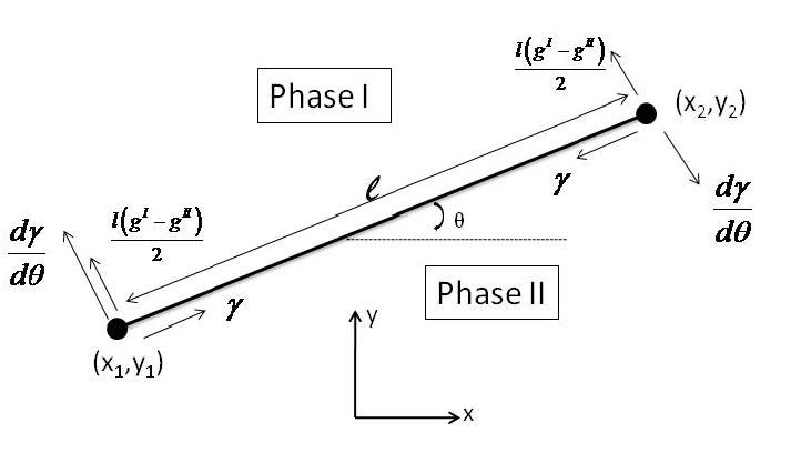
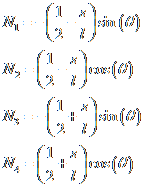
Based off of the figure, we have expressions that are used in the finite element models. The virtual motion of the interface relates to the virtual motion of nodal points by:
![]()
Where N1, N2, N3, N4 are the interpolation coefficients which are:
The interface velocity also relates to the nodal velocity as follows:
![]()
The surface tension depends on the crystalline orientation of the interface, denoted by γ(θ). When dealing with a straight element, γ is constant for each line element but will take on different values on elements of different slopes (θ). For a two dimensional structure, the total free energy is:
The first part of the summation is over all of the lengths of the element while the second is over the areas (A) of all the phases. Looking at the virtual motion of a single element, the total free energy will vary as follows:
![]()
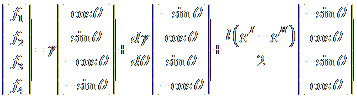
Above, gI and gII are the free energy densities of the two bulk phases and (δrn)1 and (δrn)2 are the virtual interface motions. Here we can express the free energy variation in terms of virtual motion of the nodes:
![]()
Above, f are the forces acting on the nodes. If we resolve the forces along the x and y directions, we have:
Looking at the mobility, m, may also depend on the crystalline direction. Again, for the straight line element, m is constant for that element but would vary element to element depending on slope. We can rewrite the weak statement as follows:
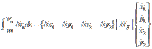
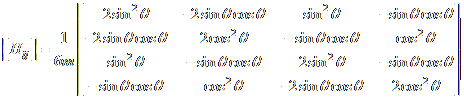
Above, [Hij] is a 4x4 matrix called the viscosity matrix. Below, [Hij] is calculated from:
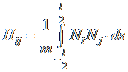
Which gives:
The weak statement becomes:
![]()
This in turn can be written as:
This is the differential equation which must be solved. Instead of trying to solve these differential equations analytically, Matlab will be used to solve these using Euler’s Method:
![]()